Muti-gene phylogeny
PhyloSuite: from data acquisition to phylogenetic tree annotation (muti-gene dataset)

In order to make it easier for users to get started, here we briefly introduce the use of PhyloSuite using an example of all available Monogenea (class) (Platyhelminthes) mitochondrial genomes (mitogenomes).
Author’s Note: To save space, the contents duplicated with our single-gene tutorial will not be detailed in this article.
1. Sequence download and preparation
Since PhyloSuite is designed both for experts and students, we will briefly introduce how to search for sequences in GenBank. We will search for all available mitogenome sequences of the class Monogenea, but this method can be applied to any other taxonomic group. After entering the NCBI’s main website (https://www.ncbi.nlm.nih.gov/), follow the steps below:
- Select the Nucleotide database;
- Enter
Monogenea[ORGN] AND (mitochondrion[TITL] OR mitochondrial[TITL]) AND 10000:50000[SLEN]into the search box. This search comprises 3 parts: first we define the target taxonomic group (Monogenea[ORGN]), then define sequence type(mitochondrion[TITL] OR mitochondrial[TITL]), and finally predefine the length range of the sequence (10000:50000[SLEN]). These keywords can be adjusted according to your needs; - Click
Send to; - Select
Complete Record --> File --> GenBankto save the complete mitogenomes. Alternatively, you may select just the Accession List (either via file or clipboard options).

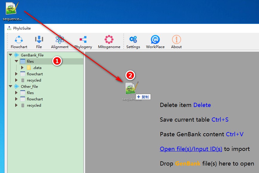
After the sequences/IDs are downloaded/copied, you can drag-drop the file directly into PhyloSuite, or click open file(s)/input ID(s) and paste the list of accession numbers there and let PhyloSuite download the selected files.
1. First select any working folder (files or flowchart);
2. Drag the file containing downloaded sequences/IDs and drop it in the area specified in the figure (display area).
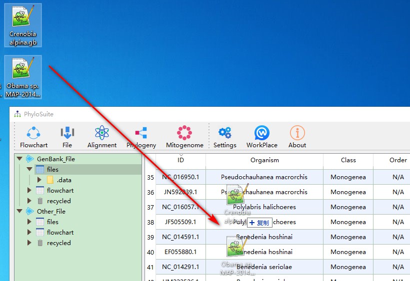
You can easily add other sequences to this dataset using the same methodology. Usually, you will have to add your own and outgroup sequence(s) separately. For this purpose, just drag them into the area shown in the figure. You may also add sequences via GB accession numbers, for which you can use add file function accessed via right-click - just paste accession number(s) into the Input IDs window, and PhyloSuite will download them automatically:
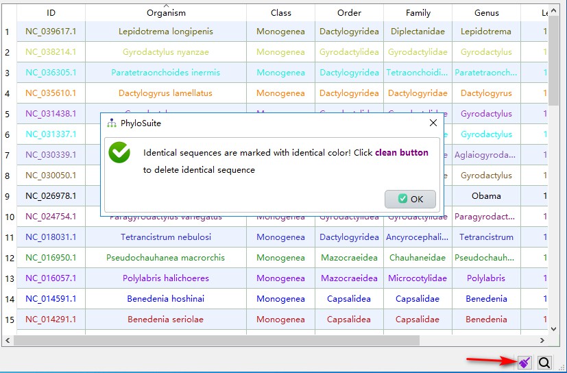
When a mitochondrial genome is uploaded to the GenBank, it will be given an accession number; after verification, it will usually be given a separate RefSeq database accession number (starting with NC). Therefore, there will be duplicate mitochondrial genomes in the downloaded data. PhyloSuite can screen them using the highlight identical sequences function (identical sequences will be marked with same colors):
1. Click the star-shaped button in the right bottom corner of the main interface, and let PhyloSuite search for duplicates;
2. If PhyloSuite identifies duplicates, the star-shaped icon will change into a purple brush. Clicking this button again will clean up the duplicates (by default, PhyloSuite preferentially retains the RefSeq IDs, starting with NC). In the demo dataset, this results in 34 retained unique sequences.
The next step is to update the lineage data (taxonomy). Use ctrl+A to select all sequences, then right-click, choose Get taxonomy (NCBI) to automatically grab the lineage information from NCBI, and then manually modify the unrecognized information. See the single gene tutorial for other details.
2. Sequence standardization
The function mainly has two aspects: the first is to standardize the synonymous gene names, and the second is to identify the problematic annotation features. For example, in mitogenomes, the two copies of trnS and trnL are commonly confused:
1. Select all sequences, then right-click and select Standardization;
2. A prompt will pop up to select the data type. Here you can select the predefined Mitogenome. You may customize the available data types (i.e., add new types or modify existent types).

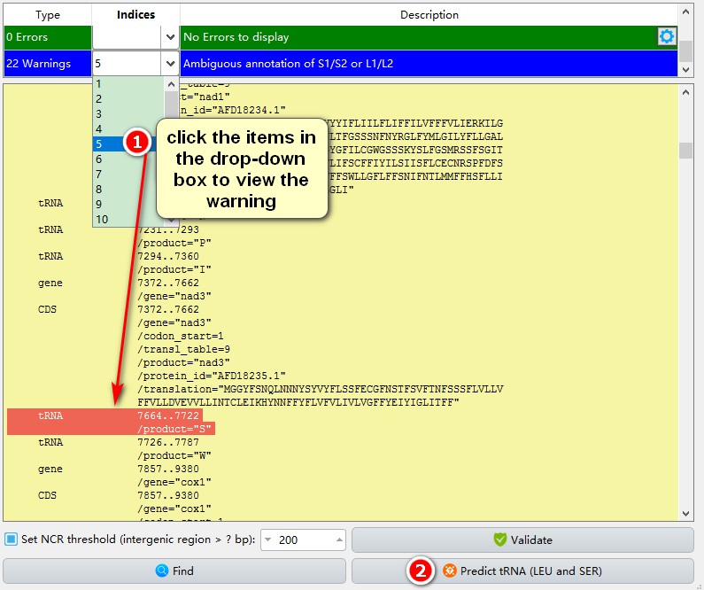
In the pop-up window, we find that there are 22 problematic trnS and trnL tRNA annotations in our dataset. If you click on the drop-down box, you can review them individually. If you intend to use only protein-coding genes (PCGs) in your analyses, you may ignore this problem, but if you are interested in the tRNA dataset, you should re-annotate them manually. PhyloSuite provides a convenient function for this:
1. Click on each item in the drop-down box to view its annotation;
2. Click on the Predict tRNA (LEU and SER) in the right bottom corner to conduct a semi-automatic ARWEN annotation.
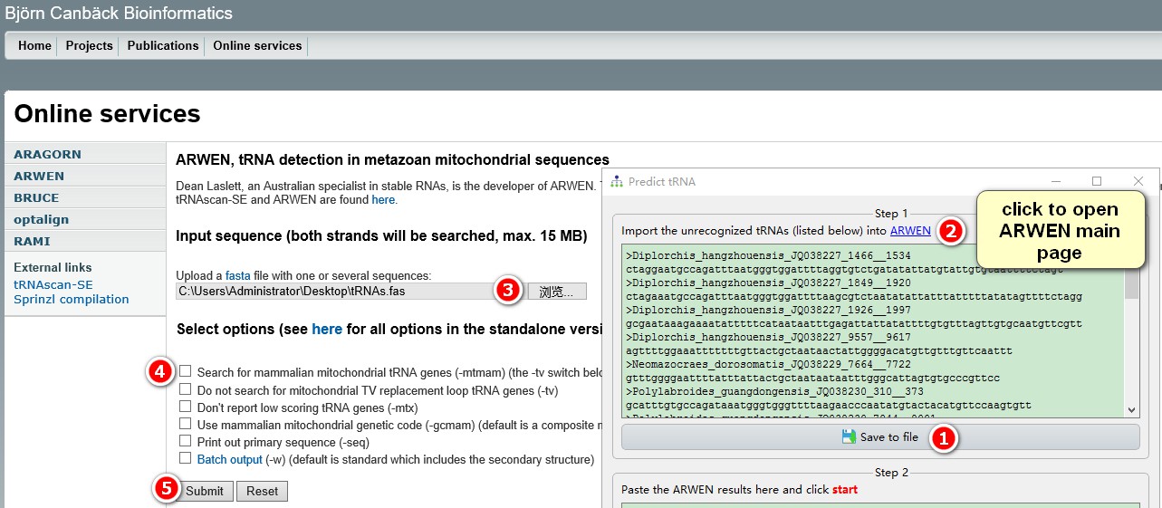
After clicking the Predict tRNA button, a window will pop up (see the figure below):
1. Save the problematic tRNA gene sequences locally via the Save to file button;
2. Click ARWEN link on the interface to open the ARWEN website. (Author’s note: this sometimes does not work if you are using the Edge browser on Win10; use this link directly: http://130.235.46.10/ARWEN/);
3. Import the file saved in the first step into ARWEN;
4. The first parameter will be selected by default. If it is not a mammalian mitochondrial genome, please uncheck it.
5. Click Submit.
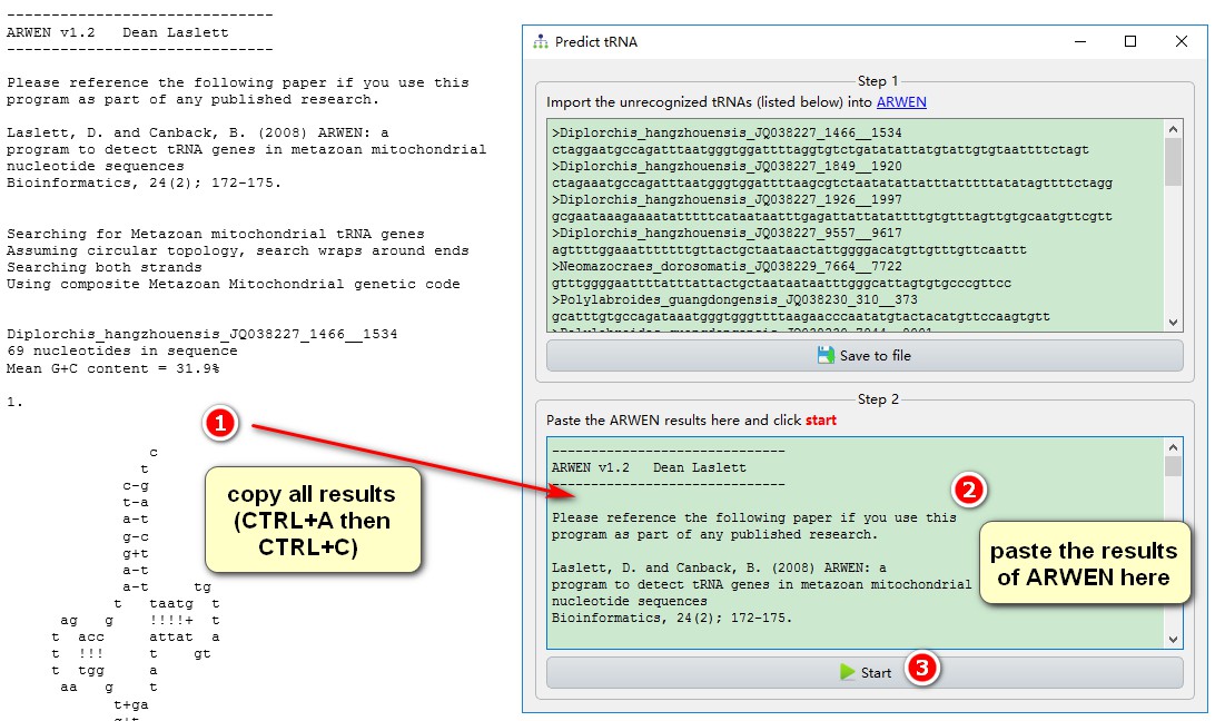
After getting the ARWEN tRNA prediction:
1. ctrl+A to select all results, and then copy them;
2. Paste the copied result into the area shown in the figure;
3. Click Start to start automatic annotation.
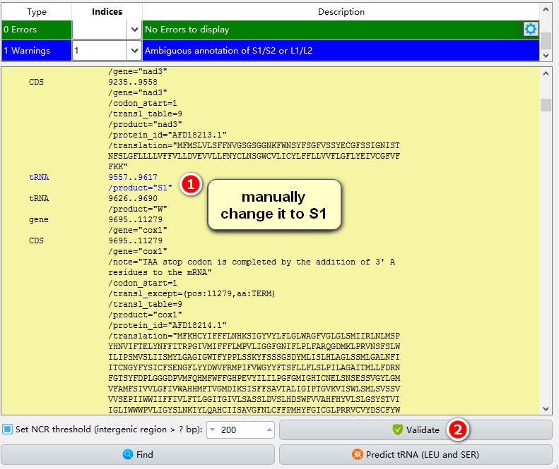
After the ARWEN annotation, there may still be some tRNAs that are not annotated successfully. If you wish, you may annotate them manually:
1. After locating the problematic annotation, I found that the problematic mitogenome had two annotated trnS2 sequences, so I changed the problematic one to S1 manually. This is a lazy way. The safest way is to use the semi-automatic step again to fetch the problematic sequences, align them both with all other homologs (trnS1 and trnS2) in the extracted results and identify them on the basis of their anti-codons and secondary structures;
2. After the modification, click Validate to save the annotation.
In addition to the above tRNA annotation issues, here are a few more examples of common errors:
If there are no feature annotations and sequences in the record, the best option is usually to delete it. You can delete it manually in this window (see below), but this is error-prone – if you don’t delete it cleanly, that is, from LOCUS to //, the program may malfunction. It is better to delete it in the main interface (display area) via the right-click menu.
The second common problem is that the specified feature does not contain default preset identifiers in the GenBank file. This happens mostly in the gene feature, because the identifiers are gene, product and note. In the screenshot below you can see that gene feature contains only locus_tag and db_xref identifiers. In this case, we can ignore this error, because the correct annotation is below, under the tRNA feature.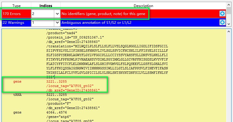
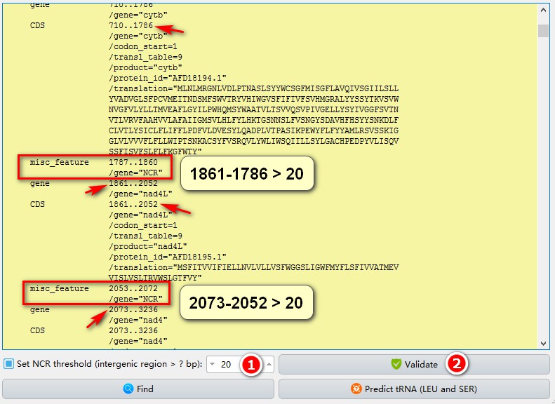
In addition to checking annotations, this feature also supports automatic labeling of non-coding regions (useful for subsequent extraction and gene sequence analyses):
1. Set the threshold for the non-coding region you wish to label and extract. When the number of intergeneric nucleotides between genes (the starting position of the downstream gene minus the end position of the upstream gene) is greater than this threshold, the intergenicspacer will be marked as a non-coding region (NCR);
2. Click Validate. In the screenshot I set the threshold to 20, and 2 intergenic regions larger than 20 bp are marked.
3. Sequence extraction
- In the main interface, select all sequences, right-click and choose
Extractto enter the extraction interface; - Monogeneans use the code table 9 (
Echinoderm and Flatworm Mitochondrial Code). Selecting the right code table is necessary to correctly identify the stop codons, translate protein-coding genes, and generate an RSCU table; - Select the predefined
Mitogenomeas the sequence type; - Set parameters for the gene order visualization in iTOL, such as the shape, color and length of each gene icon;
-
Gene Intervalis used to set the spacing between gene icons in the iTOL gene order visualization; - The content of
Lineage coloris explained in the single gene tutorial, so I won’t go into details here. Finally, clickStartto start the program.

After extraction, the sequences corresponding to each feature are stored in folders named according to corresponding GenBank file features: CDS_NUC (nucleotide sequences of genes identified within the CDS; in this case 12 genes, as atp8 is missing), CDS_AA (translated amino acid sequences of the 12 genes), rRNA (2 genes) and tRNA (22 genes). Sometimes you may encounter a situation where gene names are not standardized. For detailed procedure please refer to the single gene tutorial. Briefly: open the extract_results\StatFiles\name_for_unification.csv file, replace the name in the New Name column, then save it (csv), and finally drag this file into the extraction settings interface (see screenshot below):

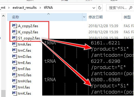
Note that there may be some sequence files with ‘copy’ in the file name in the results folder; this means that there are duplicated genes in some sequences (copy2 means 2 genes, copy3 means 3, etc.). As shown in the figure (our demo dataset doesn’t have duplicated genes, this is from another dataset just for demonstration), there are two copies of trnA, trnK and trnS1 genes in some sequences (user can open fasta files of problematic sequences to view details):
In addition to the extracted sequences, you may also find the gene order file (which can be used for CREx and TreeREx analyses) and various statistical tables in the results folder. Some of them can be used directly in your manuscript, and some can be used for downstream analyses (not shown in this tutorial).
4. Multiple sequence alignment
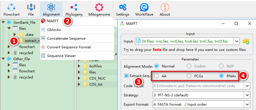
You can automatically input the results from the previous step into MAFFT in the following way (see the single gene tutorial for multiple ways of importing files):
1. Check the extract_results result folder;
2. Open MAFFT through the Alignment menu;
3. Extract-Seq is automatically checked, the sequence extracted in the extract_results folder is automatically imported into MAFFT;
4. Switch between RNAs, PCGs and AA to automatically import their corresponding sequence files.
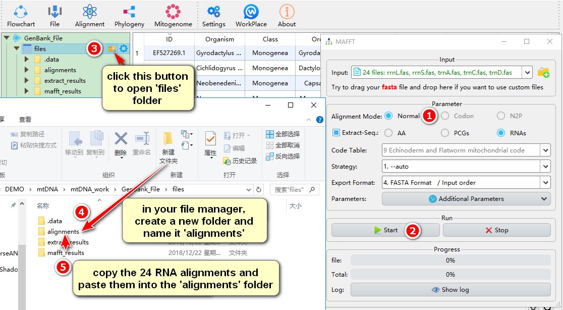
Next, batch alignment is started. Here, I selected the Normal alignment method for aligning the RNAs (22 tRNA genes + 2 rRNA genes). Ideally, the secondary structure alignment mode available in MAFFT-with-extensions should be used to align RNAs, but Windows doesn’t support it.
1. Select Normal alignment mode;
2. Other parameters can be set according to your needs, and then click Start;
3. After the alignment is complete, click the folder icon to the right of files;
4. Create a new folder named alignments within this folder;
5. Copy the 24 sequences that have just been aligned to the alignments folder, as these sequences will be overwritten when you start the next alignment.
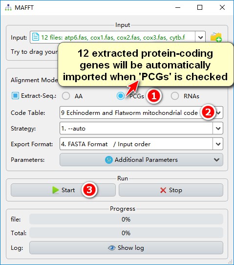
Nucleotide sequences of the PCGs should to be aligned using the codon mode (this function was added by PhyloSuite, the procedure is that the nucleotide sequences are translated into amino acid sequences, aligned by MAFFT, and then translated back into nucleotides):
1. Select PCGs to automatically import the extracted nucleotide sequence of all PCGs into MAFFT (see Input);
2. Selected the code table (9);
3. After setting other parameters, start the program.
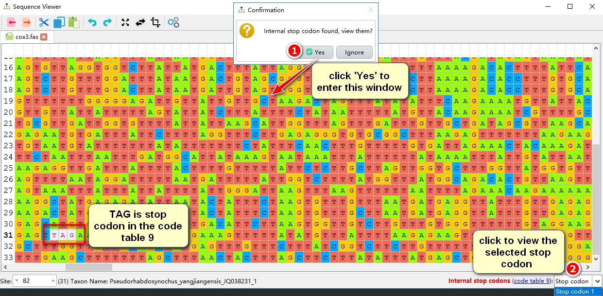
You should get a prompt that internal stop codon was found inside a gene. If you are aware of this problem, feel free to ignore it and continue the alignment, otherwise terminate the alignment and inspect the problem:
1. In the pop-up window, select Yes to view the problematic sequence;
2. Select the stop codon number in the drop-down box in the right bottom corner to view each identified internal stop codon. For example, the stop codon TAG is marked here in sequence No. 31.
Internal termination codons are commonly caused by sequencing and annotation artefacts, but if you find a very large number of internal stop codons, you probably selected a wrong code table. If you only find a few, you can ignore or delete them (if deleting, use ctrl+s to overwrite the old file, and then continue to align). Here, I ignored the internal stop codons. When the alignment is completed, copy the alignments of the 12 protein genes into the alignments folder for downstream analyses.
5. Sequence concatenation
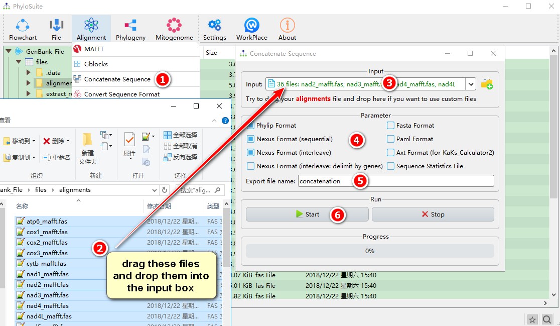
Since there are 36 aligned sequences, they need to be concatenated into a single dataset:
1. Open the Concatenation window through the Alignment menu bar (Alignment-->Concatenation);
2. Select and drag all 36 sequences in the alignments folder into the file input box.
3. You may adjust the gene order by dragging the files, but you must ensure that PCGs (12 in this case) are first, because they need to be broken down by codon positions for subsequent selection of the partition model.

- Select the format(s) of the output file;
- The name of the output file can be customized;
- Start the program.
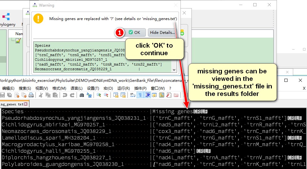
Since some species do not contain all 36 genes, there is a prompt that the missing genes will be replaced with “?”. Missing genes can be viewed in the missing_genes.txt file in the concatenate_results result folder.
6. Optimal partitioning strategy and model selection
In the next step we will use PartitionFinder2 to select the best-fit partitioning strategy and models for the concatenated sequences. Note that there is some functional overlap between this plug-in, ModelFinder and IQ-Tree, see the single gene tutorial for the other two tools. For more details about PartitionFinder2 parameters, check the manual at http://www. Robertlanfear.com/partitionfinder/assets/Manual_v2.1.x.pdf.
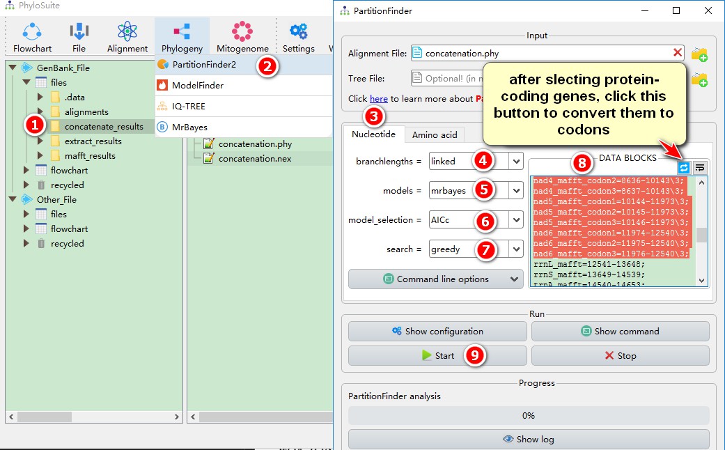
1. Select the concatenate_results folder;
2. Open Phylogeny-->PartitionFinder2 through the menu bar, and the concatenated dataset with the position index of each gene will be automatically imported;
3. Select the Nucleotide mode;
4. Select linked for branchlengths. If unlinked, MrBayes will generate separate trees for each partition, and the analysis may not converge.
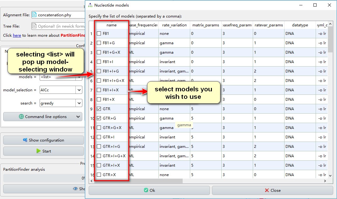
5. For models, select mrbayes; this will calculate the models supported by MrBayes. The models supported by RAxML can be set by --raxml in Command line options. Currently, there is no predefined IQ-TREE support, so you can select all, or <list> to customize models (see screenshot below):
6. AICc is the model selection criterion recommended by the PartitionFinder author;
7. search method, you can choose greedy;
8. DATA BLOCKS sets the position index for each gene, as sometimes we need to split the PCGs by codon positions to calculate the optimal partitioning strategy, and models for each codon site. Select 12 protein genes, then use the conversion button (shown in the screenshot) to split them by codon positions. Press the button again to revert back (Note: all the protein genes must be listed together and at the beginning of the concatenated dataset);
9. Other parameters can be set according to your own needs, and then start the program.
7. Phylogenetic tree reconstruction based on the Bayesian method (BI)
Consequently, we can use the results of PartitionFinder2 to reconstruct the phylogenetic tree using Bayesian method:
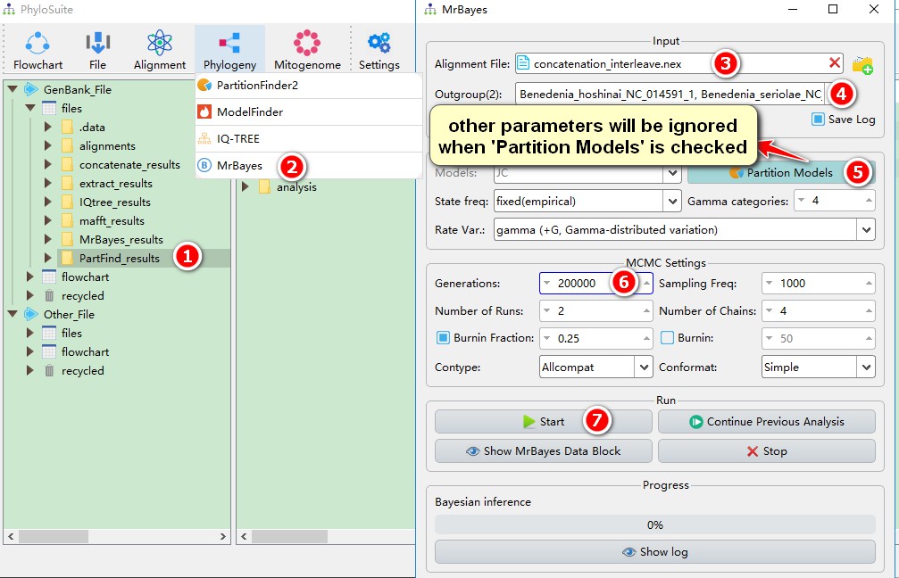
1. Select the PartFind_results folder;
2. Open the Phylogeny-->MrBayes via the menu bar, PartitionFinder2 results will be automatically imported;
3. The sequence file in the PartitionFinder2 result will be automatically converted to NEXUS format (interleave mode) as the input file for MrBayes. If it is not interleaved, there is a length limit of 99990 characters;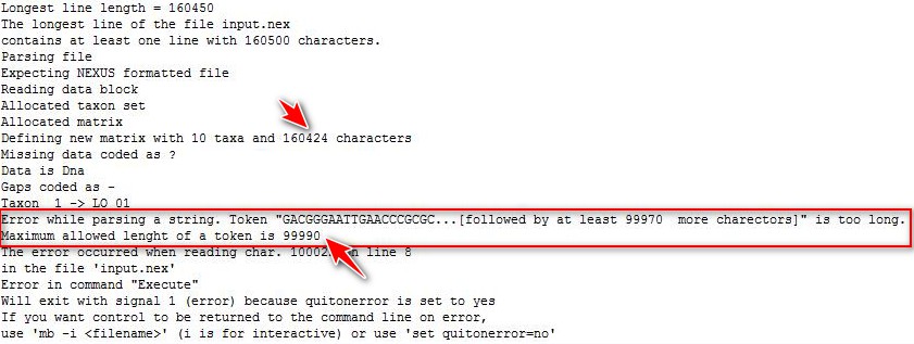
4. The outgroup can be selected through the drop-down menu (multiple outgroups can be set);
5. Since we use the results of PartitionFinder2, the Partition Models mode will be automatically selected, and settings for some other model parameters, such as State freq, will be ignored;
6. Set the number of generations;
7. Play with other parameters if you wish, and then start the program.
8. Maximum likelihood method (ML) phylogenetic tree reconstruction
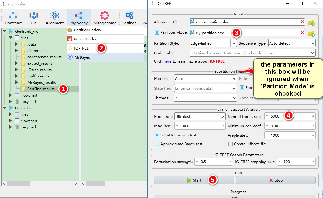
Similar to MrBayes, the results of PartitionFinder2 can be directly used by IQ-TREE:
1. Select the PartFind_results result folder;
2. Open Phylogeny-->IQ-TREE through the menu bar. The result of PartitionFinder2 is automatically imported;
3. When using PartitionFinder2, the Partition Mode will be automatically selected, and the parameter settings in the Substitution Model Options section will be ignored;
4. For relatively large datasets you can use the Ultrafast bootstrap method introduced by IQ-TREE, but the number of replicates should be relatively large (minimum 5000). If you choose Standard, it will be slower;
5. Play with other parameters if you wish, and then start the program.
9. Flowchart
When you use datasets comprised of PCGs and RNAs (e.g., all 36/37 mitochondrial genes), it is best to use different alignment modes, and the codon sites of the PCGs need to be tested (partitioning+models), so it is best to use the procedure described so far. However, if you want to reconstruct a phylogenetic tree using just PCGs (regardless of whether you wish to use amino acids or nucleotides), you can use Workflow function to complete the entire phylogenetic analysis operation in one step. The execution order of the workflow is: alignment –> removal of poorly aligned sections (optional) –> concatenation –> partitioning and model selection –> phylogeny reconstruction (Bayesian/maximum likelihood method). You only have to select input files for the first program (MAFFT), as all downstream programs will automatically use the output of the upstream program as input file (see also the single gene tutorial):
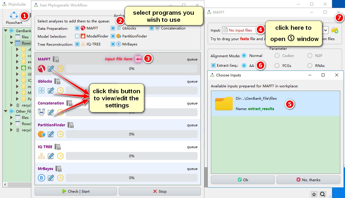
1. Click Flowchart in the menu bar;
2. Select the desired analyses; here we will use MAFFT, Gblocks, Concatenation, PartitionFinder, IQ-TREE (ML) and MrBayes (BI);
3. As stated above, you only need to input the file in the first program, so click the red Input file here to open the MAFFT program window;
4. Click the file input box of MAFFT to view the automatically prepared input files (you may opt to use a different file via No, thanks);
5. Select the results that you extracted in section 3 (extract_results);
6. Extract-Seq option select AA, and the amino acid sequences will be imported automatically;
7. Just close the window to save the imported files.
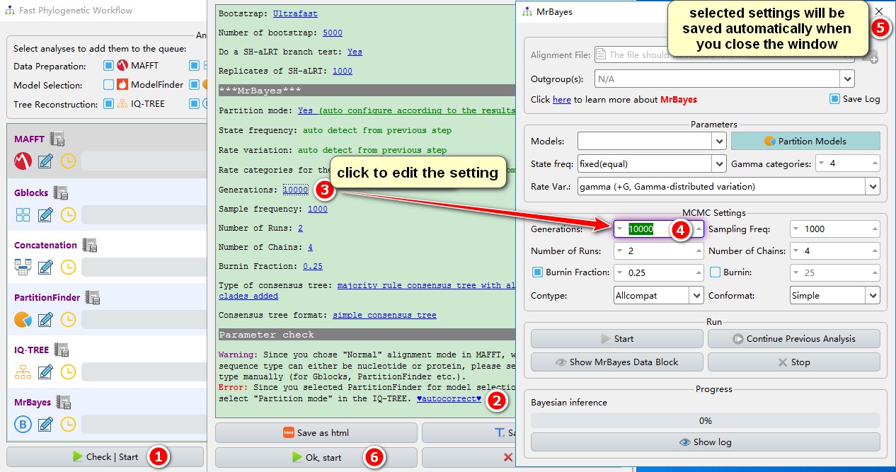
You may click the edit button next to each function pane (shown in the screenshot above) to set the parameters of each program, or modify the parameters in the parameter summary window (recommended), as follows (see also the single gene tutorial):
1. Click the Check | Start button, and the parameter summary window will pop up, allowing you to check and modify the parameters;
2. PhyloSuite is able to automatically check for conflicting parameters. For example, because PartitionFinder is used, partition mode should be checked in IQ-TREE. Clicking the blue ‘autocorrect’ function will automatically complete this operation;
3. If you wish to edit any of the settings (blue letters), just click on them…
4. …and the corresponding settings window will pop up, with the widget you wish to edit highlighted;
5. After setting the parameters for each software, they will be automatically saved when you close the window;
6. Click Ok, start to start the Flowchart.
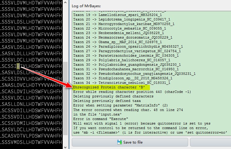
You will notice that MrBayes reports and error. This is caused by an unrecognized character B in one of the sequences in our dataset, it is an annotation error in that GenBank record. Open the sequence viewer or input file, find the rogue character, and delete it:
After all the programs have finished, the main interface will display the summary of materials & methods and references (also see the single gene tutorial).
10. Phylogenetic Tree Annotation
Finally, we will introduce the annotation of the phylogenetic tree, as PhyloSuite generates many files useful for this:
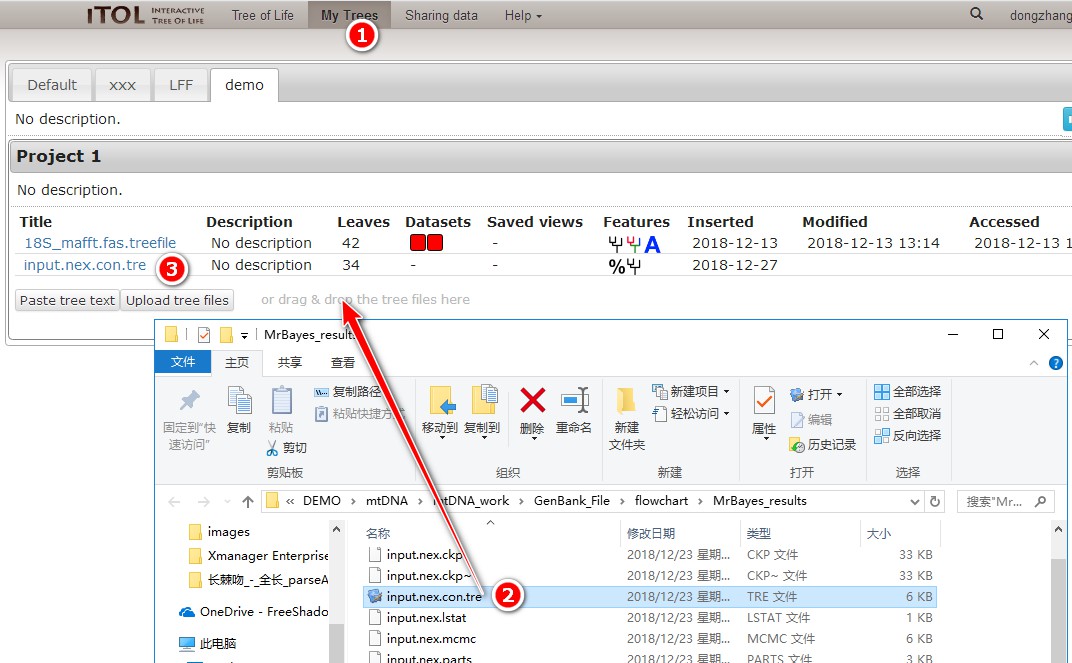
1. First, open iTOL’s home page https://itol.embl.de/, log into your account, and select My Trees;
2. Double-click MrBayes_results to open the result of MrBayes, and drag the *.con.tre file into the area shown in the figure to import it automatically;
3. Click on the tree to enter the editing interface.
- Support value can be displayed using the tab
Advanced;

In PhyloSuite, double-click
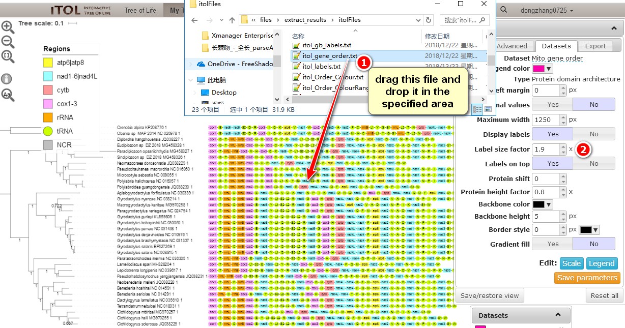
extract_resultsto open the extraction step results (section 3). Open theitolFilesfolder, which contains files useful for the iTOL phylogram annotation. Just drag the file into iTOL interface to see what happens. Batch replacement of species names and marking taxa with colors are described in the single gene tutorial, so here we mainly focus on mapping gene orders to phylogenetic trees;
a. Drag theitol_gene_order.txtfile into the iTOL interface;
b. In theDatasetstab you can play with different settings, such asLabel size factorto control the font size of each gene name.
Since there are many files that can be used for tree annotation, you can combine them into a variety of annotation effects. Here we demonstrate one:
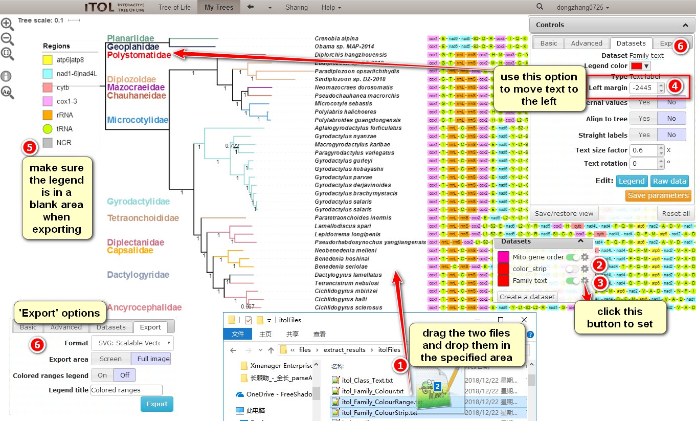
a. Dragitol_Family_ColourRange.txtanditol_Family_ColourStrip.txtto annotate the families;
b. Closecolor_strip, as we only need this function to colorize the branches (they remain colorized even after you uncheck the strip);
c. Click on the gear icon of theFamily textto change settings;
d. Move the text of the section to the left by adjusting theLeft marginvalue, whereas text size can be changed via theText size factor;
e. Place the legend in a blank area before exporting the tree, as this makes subsequent editing easier;
f. Select theExporttab to export the annotated phylogenetic tree (useSVGformat if you intend to use Adobe Illustrator).
Finally, you can use Adobe Illustrator (or other suitable software) to make final adjustments to the image, such as adjusting the position of the family name, the location of the legend, and adding gradient color blocks:
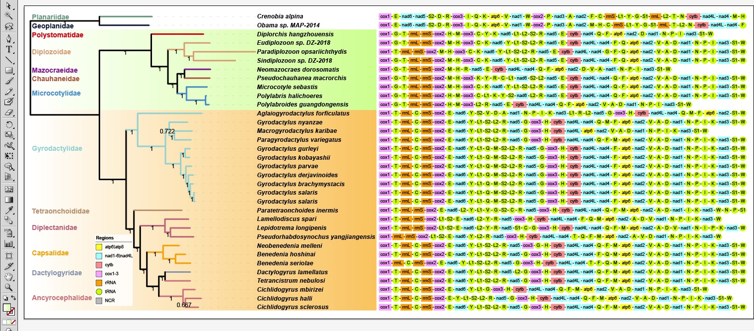
By the way,
The advantages of this annotation method are especially pronounced when you have hundreds of species, or when you want to compare multiple topologies based on the same dataset. Colourated annotation is very helpful in such cases, especially for identifying paraphyly and polyphyly.
11. Software download address
https://github.com/dongzhang0725/PhyloSuite/releases or http://phylosuite.jushengwu.com/dongzhang0725.github.io/installation/#Chinese_download_link (China)
12. Reference
Zhang, D., F. Gao, I. Jakovlić, H. Zou, J. Zhang, W.X. Li, and G.T. Wang, PhyloSuite: An integrated and scalable desktop platform for streamlined molecular sequence data management and evolutionary phylogenetics studies. Molecular Ecology Resources, 2020. 20(1): p. 348–355. DOI: 10.1111/1755-0998.13096.